38 how to display data labels in excel chart

Format Data Labels in Excel- Instructions - TeachUcomp, Inc. To do this, click the "Format" tab within the "Chart Tools" contextual tab in the Ribbon. Then select the data labels to format from the "Chart Elements" drop-down in the "Current Selection" button group. Then click the "Format Selection" button that appears below the drop-down menu in the same area. Excel 2010: Show Data Labels In Chart - AddictiveTips To enable data labels in chart, select the chart and head over to Chart Tools Layout tab, from Labels group, under Data Labels options, select a position. It will show Data labels at specified position. Likewise, from Data Labels pull-down menu, you can change the position of data labels and access other advance options.

Excel charts: add title, customize chart axis, legend and data labels ... Click the Chart Elements button, and select the Data Labels option. For example, this is how we can add labels to one of the data series in our Excel chart: For specific chart types, such as pie chart, you can also choose the labels location. For this, click the arrow next to Data Labels, and choose the option you want.

How to display data labels in excel chart

› documents › excelHow to add data labels from different column in an Excel chart? Right click the data series in the chart, and select Add Data Labels > Add Data Labels from the context menu to add data labels. 2. Click any data label to select all data labels, and then click the specified data label to select it only in the chart. 3. How to add data labels from different column in an Excel chart? This method will guide you to manually add a data label from a cell of different column at a time in an Excel chart. 1.Right click the data series in the chart, and select Add Data Labels > Add Data Labels from the context menu to add data labels.. 2. How to Use Cell Values for Excel Chart Labels Select the chart, choose the "Chart Elements" option, click the "Data Labels" arrow, and then "More Options." Uncheck the "Value" box and check the "Value From Cells" box. Select cells C2:C6 to use for the data label range and then click the "OK" button. The values from these cells are now used for the chart data labels.

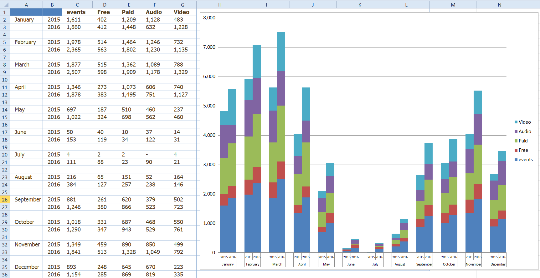
How to display data labels in excel chart. Chart: Display alternative values as Data Labels or Data Callouts Joined. Aug 11, 2017. Messages. 1. Aug 11, 2017. #1. Below is my excel chart. I would like to add a "data labels" or "data callouts". As you can see the line is displaying the data from Actual X and Y, but I want to display the DEV values on this line. How to Create a Bar Chart With Labels Above Bars in Excel In the chart, right-click the Series "# Footballers" Data Labels and then, on the short-cut menu, click Format Data Labels. 9. In the Format Data Labels pane, under Label Options selected, set the Label Position to Inside Base. 10. Then, under Label Contains, check the Category Name option and uncheck the Value and Show Leader Lines options. 11. How to Add Labels to Show Totals in Stacked Column Charts in Excel Press the Ok button to close the Change Chart Type dialog box. The chart should look like this: 8. In the chart, right-click the "Total" series and then, on the shortcut menu, select Add Data Labels. 9. Next, select the labels and then, in the Format Data Labels pane, under Label Options, set the Label Position to Above. 10. Add / Move Data Labels in Charts - Excel & Google Sheets Adding Data Labels Click on the graph Select + Sign in the top right of the graph Check Data Labels Change Position of Data Labels Click on the arrow next to Data Labels to change the position of where the labels are in relation to the bar chart Final Graph with Data Labels

Adding Data Labels to Your Chart (Microsoft Excel) - tips To add data labels, follow these steps: Activate the chart by clicking on it, if necessary. Choose Chart Options from the Chart menu. Excel displays the Chart Options dialog box. Make sure the Data Labels tab is selected. (See Figure 1.) The left side of the dialog box shows the different types of data labels you can choose. (The available ... Select Data to Display in an Excel Chart With Option Buttons Feb 17, 2015 · You could put the chart and option buttons on the active sheet, and all of the data (and the option button linked cell) can go onto another sheet, and you can hide this other sheet if you want. Or you can place the original data on the same sheet as the chart and option buttons, and the formulas onto another sheet, a hidden sheet if desired. How to Customize Your Excel Pivot Chart Data Labels - dummies The Data Labels command on the Design tab's Add Chart Element menu in Excel allows you to label data markers with values from your pivot table. When you click the command button, Excel displays a menu with commands corresponding to locations for the data labels: None, Center, Left, Right, Above, and Below. None signifies that no data labels ... › documents › excelHow to display text labels in the X-axis of scatter chart in ... Actually, there is no way that can display text labels in the X-axis of scatter chart in Excel, but we can create a line chart and make it look like a scatter chart. 1. Select the data you use, and click Insert > Insert Line & Area Chart > Line with Markers to select a line chart. See screenshot: 2. Then right click on the line in the chart to ...

Text Labels on a Horizontal Bar Chart in Excel - Peltier Tech Dec 21, 2010 · In Excel 2003 the chart has a Ratings labels at the top of the chart, because it has secondary horizontal axis. Excel 2007 has no Ratings labels or secondary horizontal axis, so we have to add the axis by hand. On the Excel 2007 Chart Tools > Layout tab, click Axes, then Secondary Horizontal Axis, then Show Left to Right Axis. How to show data label in "percentage" instead of - Microsoft Community Select Format Data Labels. Select Number in the left column. Select Percentage in the popup options. In the Format code field set the number of decimal places required and click Add. (Or if the table data in in percentage format then you can select Link to source.) Click OK. Regards, OssieMac. Report abuse. Outside End Labels - Microsoft Community Replied on February 16, 2018. Hi Watson, Outside end label option is available when inserted Clustered bar chart from Recommended chart option in Excel for Mac V 16.10 build (180210). As you mentioned, you are unable to see this option, to help you troubleshoot the issue, we would like to confirm the following information: How to use data labels in a chart - YouTube Excel charts have a flexible system to display values called "data labels". Data labels are a classic example a "simple" Excel feature with a huge range of o...

Example: Charts with Data Tools — XlsxWriter Documentation

Understanding Excel Chart Data Series, Data Points, and Data Labels Sep 19, 2020 · Numeric Values: Taken from individual data points in the worksheet.; Series Names: Identifies the columns or rows of chart data in the worksheet. Series names are commonly used for column charts, bar charts, and line graphs. Category Names: Identifies the individual data points in a single series of data.These are commonly used for pie charts.

Pie Chart - PK: An Excel Expert

support.microsoft.com › en-us › officeAdd or remove data labels in a chart - support.microsoft.com Click the data series or chart. To label one data point, after clicking the series, click that data point. In the upper right corner, next to the chart, click Add Chart Element > Data Labels. To change the location, click the arrow, and choose an option. If you want to show your data label inside a text bubble shape, click Data Callout.

How to Make an Excel Histogram Display the Data Distribution - My Microsoft Office Tips

Excel tutorial: How to use data labels Generally, the easiest way to show data labels to use the chart elements menu. When you check the box, you'll see data labels appear in the chart. If you have more than one data series, you can select a series first, then turn on data labels for that series only. You can even select a single bar, and show just one data label.

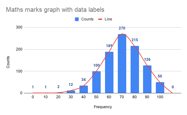
Part 2: Creating a Histogram with Data Labels and Line Chart | by Bhavesh Parvatkar | Udacity ...

Change the format of data labels in a chart To get there, after adding your data labels, select the data label to format, and then click Chart Elements > Data Labels > More Options. To go to the appropriate area, click one of the four icons ( Fill & Line, Effects, Size & Properties ( Layout & Properties in Outlook or Word), or Label Options) shown here.

GANTT Procedure

Add a DATA LABEL to ONE POINT on a chart in Excel Click on the chart line to add the data point to. All the data points will be highlighted. Click again on the single point that you want to add a data label to. Right-click and select ' Add data label ' This is the key step! Right-click again on the data point itself (not the label) and select ' Format data label '.

MS Excel 2013: Display the fields in the Values Section in a single column in a pivot table

How to Make a Bubble Chart in Microsoft Excel Create the Bubble Chart. Select the data set for the chart by dragging your cursor through it. Then, go to the Insert tab and Charts section of the ribbon. Advertisement. Click the Insert Scatter or Bubble Chart drop-down arrow and pick one of the Bubble chart styles at the bottom of the list.

Friday Challenge Answers: Year over Year Chart Comparisons - Excel Dashboard Templates

Create Dynamic Chart Data Labels with Slicers - Excel Campus Feb 10, 2016 · Typically a chart will display data labels based on the underlying source data for the chart. In Excel 2013 a new feature called “Value from Cells” was introduced. This feature allows us to specify the a range that we want to use for the labels. Since our data labels will change between a currency ($) and percentage (%) formats, we need a ...

Working with Multiple Data Series in Excel | Pryor Learning Solutions

How To Make A Bubble Chart In Microsoft Excel | CodePre.com Create the bubble chart. Select the data set for the chart by dragging the cursor across it. Then go to the Insert tab and the Graphics section of the ribbon. Click the Insert scatter or bubble chart drop-down arrow and choose one of the bubble chart styles at the bottom of the list.

Share :